

Looking for ways for automated data cleaning in Excel? Then, this is the right place for you. Sometimes, the data we get is not clean and ready for analysis. In those cases, we need to clean and prepare data by following some steps. Here, you will find 10 different step-by-step explained ways to get knowledge about automated data cleaning in Excel.
10 Ways for Automated Data Cleaning in Excel
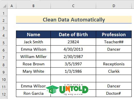
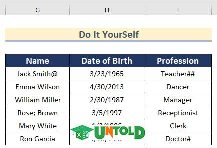
Here, we have a disorganized dataset containing Name, Date of Birth, and Profession of some people. Now, we will show you ways for automated data cleaning in Excel using this dataset.
1. Use of Power Query Feature to Clean Data in Excel
In the first method, we will use the Power Query Feature for automated data cleaning. Follow the steps to do it on your own dataset.
Steps:
- Firstly, select Cell range B4:D10.
- Then, go to the Data tab >> click on From Table/Range.

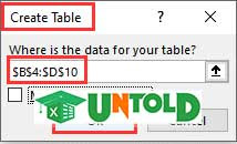
- Now, the Create Table box will open and the dataset has already been selected.
- After that, press OK.
- Next, the Power Query Editor will appear.
- Then, click on Use First Row as Headers to set the header.

- Afterward, to change the text case, select the Name column.
- Now, go to the Transform tab >> click on Text Column >> click on Format >> select Capitalize Each Word.

- Next, click on the button below to remove rows with empty cells.
- After that, click on Remove Empty.

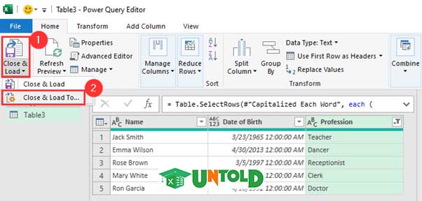
- Then, click on Close & Load >> select Close & Load To.
- Now, the Import Data box will open.
- Next, select the New worksheet option.
- After that, click on OK.

- Thus, you can clean data automatically using Power Query Editor.

2. Applying Text to Columns Feature in Excel
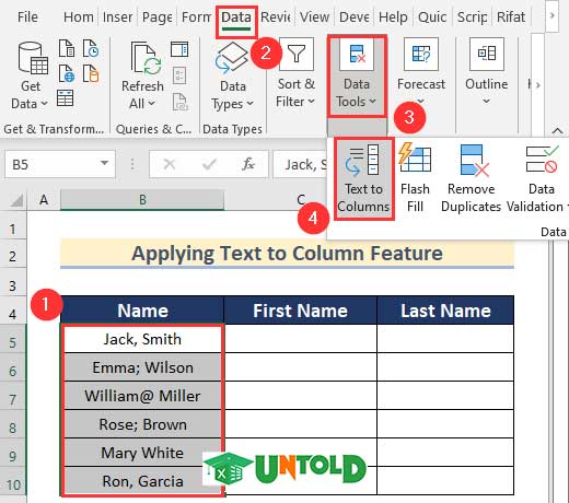
Here, in the dataset, we have both the first and last name of a person in the same column titled as Name. We can separate the data into two different columns using the Text to Columns feature for automated data cleaning in Excel.
Here are the steps.
Steps:
- In the beginning, select Cell range B5:B10.
- Then, go to the Data tab >> click on Data Tools >> select Text to Columns.
- After that, click on Next.

- Next, select Semicolon, Comma, Space and @ in Others as Delimiters.
- Then, click on Next.

- Now, insert Cell C5 as Destination.
- After that, click on Finish.

- Finally, you can see that the data have been divided into two columns First Name and Last Name.

Read More: How to Remove Partial Data from Multiple Cells in Excel
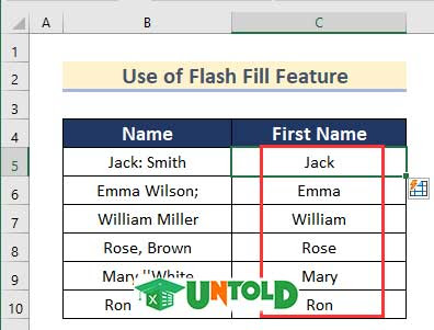
3. Use of Flash Fill Feature for Automated Data Cleaning in Excel
Now, you will find a way to use the Flash Fill Feature for automated data cleaning in Excel. Here, we have different unwanted symbols in the dataset. You can remove them by following the steps given below.
Steps:
- Firstly, insert Jack in the First Name column.
- After that, go to the Data tab >> click on Data Tools >> click on Flash Fill.
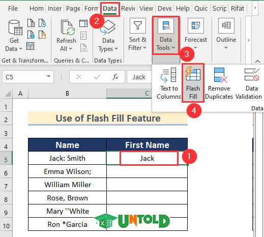
- Now, you will see that all the other symbols have been removed.
4. Use of SUBSTITUTE Function for Data Cleaning in Excel
Next, we will show you how you can remove unwanted symbols for automated data cleaning in Excel using the SUBSTITUTE function.

Follow the steps given below to do it on your own.
Steps:
- In the beginning, select Cell D5.
- Then, insert the following formula.

Here, in the SUBSTITUTE function, we inserted Cell C5 as text, “@” as old_text and blank (“ “) as new_text.
- After that, press ENTER and drag down the Fill Handle tool to AutoFill the formula for the rest of the cells.

- Finally, the SUBSTITUTE function has removed the unwanted symbols from column D.
5. Applying Find & Replace Feature in Excel
In the fifth method, we will clean data using the Find and Replace option in Excel. Here, we can see two values containing “#” and two values containing “@” and “;”. We will replace this value with blank by applying Find and Replace option.

Steps:
- First, select Cell range B5:D10.
- Then, go to the Home tab >> click on Editing >> click on Find & Select >> select Replace.

- Now, the Find and Replace toolbox will open.
- Next, insert “#” in the Find what box and blank in the Replace with box.
- After that, click on Replace.

- Then, you will see that “#” has been removed.

- Similarly, you can remove “@” and “;” from the dataset using the Find & Replace Feature.

Read More: Using Excel to Clean and Prepare Data for Analysis
6. Using Number Format for Automated Data Cleaning in Excel
Now, you will learn how to change Number Format for automated data cleaning in Excel. Here, some of the values of the Date of Birth are not in Date format. Go through the steps given below to clean data on your own.
Steps:
- Firstly, select Cell range C5:C10.
- Then, go to the Home tab >> click on Number Format >> click on the drop-down button.

- After that, select Short Date.

- Thus, you can change the Number Format of the dataset to clean data automatically in Excel.

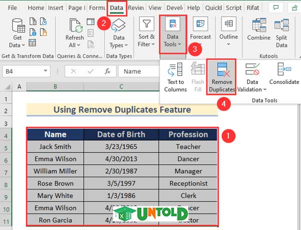
7. Using Remove Duplicates Option for Data Cleaning
Now, we will remove the duplicate values by using the Remove Duplicates feature for automated data cleaning in Excel.

Steps:
- Firstly, select Cell range B4:D11.
- Then, go to the Data tab >> click on Data Tools >> select Remove Duplicates.
- Now, the Remove Duplicates dialog box will open.
- After that, press OK.

- Next, another box containing the information of the duplicates will appear.
- Then, press OK.

- Finally, the Remove Duplicates feature will remove the duplicate values from the dataset.

Read More: How to Clean Up Raw Data in Excel
8. Applying Go To Special Feature for Automated Data Cleaning
Now, we will use the Go to Special feature to detect blank cell ways for automated data cleaning in Excel.

Here are the steps.
Steps:
- In the beginning, select Cell range B4:D11.
- Then, go to the Home tab >> click on Editing >> click on Find & Select >> select Go To Special.

- Now, the Go To Special box will appear.
- After that, select Blanks.
- Next, click on OK.

- Then, you will see that the blank cells have been selected.

- Now, you can change the format of the selected cells according to your choice.
- Here, we will go to the Home tab >> click on Fill Color >> select Red as Fill Color.

- Thus, you can detect blank cells to clean data in Excel automatically.

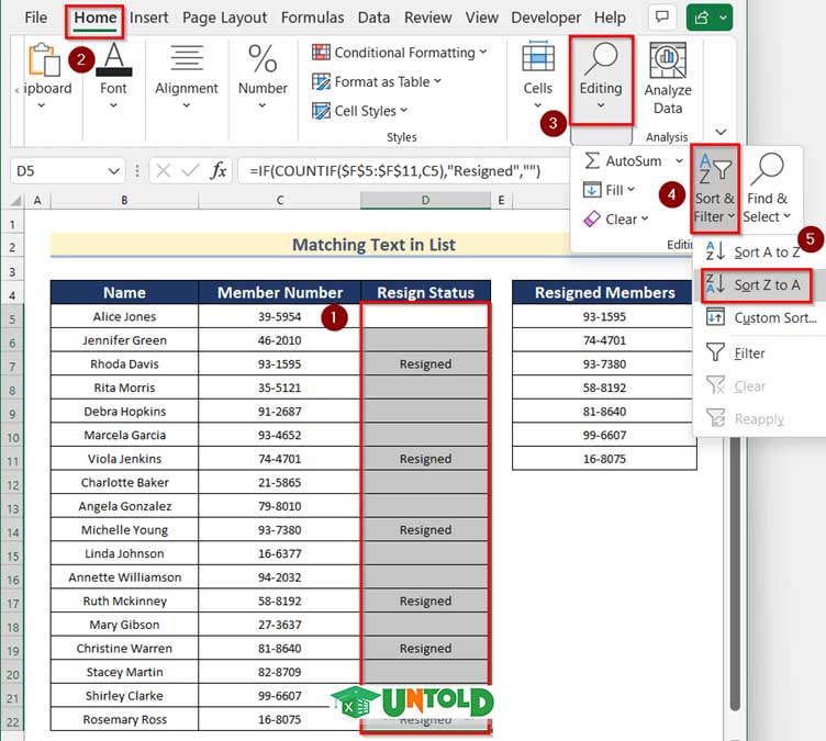
9. Matching Text in List for Data Cleaning in Excel
You may have some data and you want to check this data against another available list. See the following screenshot of our example. We are going to find out the persons who have resigned from the left side of our example. There is a list on the right side of the resigned numbers.

The above screenshot shows a simple example. The data is in the range B5:D22. The goal is to identify the rows in the data zone which are appearing in the Resigned Members list, in column F. You can delete these unnecessary rows later.
Steps:
- Firstly, select Cell D5.
- Then, insert the following formula.

Here, the COUNTIF function of the formula will return 1 if it (bold part) matches a list value(Cell range F5:F11) with a data value (Cell C5). If this part returns 1 or more, then the IF function will return “Resigned”, otherwise nothing.
- After that, press ENTER and drag down the Fill Handle tool to AutoFill the formula for the rest of the cells.

This whole formula will display the word “Resigned” if the “Member Num” in column C is found in the “Resigned Members” list. If the Member number is not found, it returns an empty string.
- Now, this whole formula will display the word “Resigned” if the “Member Num” in column C is found in the “Resigned Members” list. If the Member number is not found, it returns an empty string.

You can sort the list by column D, the rows for all Resigned Members will appear together and can be quickly deleted.
- To sort by column D, just select Cell D5 to D22.
- Then, choose Home⇒Editing⇒Sort & Filter ⇒ Sort Z to A.
- Next, the Sort Warning box will open.
- After that, select Expand the selection.
- Now, click on Sort.

- Then, our Excel sample file will be like this one.

This technique can be adapted to other types of list-matching tasks.
Read More: How to Clean Survey Data in Excel
10. Using Spell Check for Cleaning in Excel
In the final step, we will show you how to Spell Check for automated data cleaning in Excel. Follow the steps given below to do it on your own.
Steps:
- In the beginning, select Cell range C5:C10.
- Then, to go to the Review tab >> click on abc Spelling.

- Now, the Spelling box will open.
- After that, select Manager.
- Then, click on Change.

- Next, select Receptionist.
- Afterward, click on Change.

- Now, select Clerk.
- After that, select Change.

- Next, a Microsoft Excel warning box will appear.
- Then, click on OK.

- Thus, you can use Spell Check to clean data in Excel.

Practice Section
In the article, you will find an Excel workbook like the image below to practice independently.
Download Practice Workbook
Conclusion
So, in this article, we have shown you ways for automated data cleaning in Excel. I hope you found this article interesting and helpful. If something seems difficult to understand, please leave a comment. Please let us know if there are any more alternatives that we may have missed. Thank you!
No comments:
Post a Comment