

For those of you who have started learning Excel, we have some good news for you. In this article, we’ll discuss all your queries regarding what is active cell in Excel. In addition, we’ll see how to select, change, format, and highlight the active cell using Excel options, shortcuts, and VBA code.
What Is an Active Cell in Excel: A Complete Guide
An active cell, also known as a cell pointer or selected cell, refers to a cell in the Excel spreadsheet that is currently in selection. Typically, an active cell has a thick border around it.
Each cell in Excel has a unique address which is denoted by a column letter and row number, for instance, the address of the C7 cell is shown in the image below.
📄 Note: The letter (C) refers to the Columns while the number (7) represents the Rows.
Now, a worksheet in Excel contains around 17 billion cells and the last cell in the worksheet has the address XFD1048576. Here, XFD is the Column letter whereas 1048576 is the Row number.

Changing Active Cell in Excel
In this portion, we’ll learn how to navigate an Excel worksheet, so let’s begin.
In order to change the active cell, you can use the Arrow keys (Up, Down, Left, and Right) on your keyboard or you can Left-click your mouse to jump into any cell.
For example, if you hit the right Arrow key the active cell will move to the right of the current active cell.

Next, the address of the currently active cell is shown in the Name Box in the top-left corner.

Selecting Excel Multiple Cells as Active Cell
Generally speaking, you can select multiple cells in a spreadsheet, however, there can be only one active cell at a time. Here, although we’ve chosen multiple cells (B5:D9), only the B5 cell is active.

Now, to make our life easier, Excel has a nifty trick to populate multiple rows at once with a specific value or text. So, just follow these steps.
📌 Steps:
- Firstly, select a range of cells, here, we’ve selected the B5:D9 cells.
- Now, type in a text or any value in the Formula Bar which in this case is, ExcelUntold.
- Lastly, press the CTRL + ENTER keys on your keyboard.

The result should look like the image shown below.

Formatting Active Cell in Excel
Admittedly, we haven’t discussed how to enter a value into a cell, hence let us see the process in detail.
📌 Steps:
- Initially, press the F2 key or Double-click the left button on the mouse to enter into the Edit Mode in Excel.

- Then, type in a value or text like ExcelUntold and press the ENTER key.

That’s it you’ve placed text into a cell.
Now, that we’ve learned to navigate and enter data in Excel, our next priority would be to Format the cells according to our preferences. So, let’s take a deep dive into this matter.
1. Using Format Cells Dialog Box
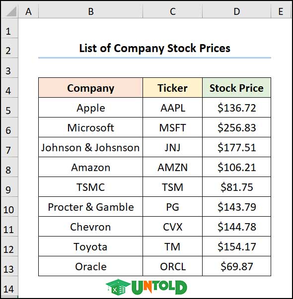
Considering the List of Company Stock Prices dataset shown in the B4:D13 cells. Here, the dataset shows the Company name, its Ticker, and the Stock Price respectively.
Now, we want to format the Stock Price column to show the prices in USD.

📌 Steps:
- First and foremost, select the D5:D13 cells >> Right-click the mouse button to open the list >> choose Format Cells options.

Now, this opens the Format Cells dialog box.
- Next, click the Number tab >> in the Currency section, select 2 Decimal places >> hit OK.

Eventually, this formats the Stock Prices in the USD.
2. Using Keyboard Shortcut
Wouldn’t it be great if only there was a keyboard shortcut to Format Cells? Well, you’re in luck because the next method answers your question. So, let’s see it in action.
📌 Steps:
- First of all, select the D5:D13 cells >> press the CTRL + 1 keys.

Now, this opens the Format Cells wizard.
- In turn, click the Number tab >> go to the Currency section and select 2 Decimal places >> press the OK button.

Consequently, this formats the Stock Prices in the USD as shown in the image below.

3. Applying VBA Macro Tool
If you often need to format a column into currency, then you may consider the VBA code below. It’s simple & easy, just follow along.
📌 Steps:
- Firstly, navigate to the Developer tab >> click the Visual Basic button.

This opens the Visual Basic Editor in a new window.
- Secondly, go to the Insert tab >> select Module.

For your ease of reference, you can copy the code from here and paste it into the window as shown below.

⚡ Code Breakdown:
Now, I will explain the VBA code used to generate the table of content.
- In the first portion, the sub-routine is given a name, here it is Format_Cell().
- Next, use the ActiveSheet property to activate the worksheet, in this case, Using VBA Code.
- Then, utilize the Range.Select method to specify the column that you want to format.
- Finally, enter the NumberFormat property to get the result in USD.

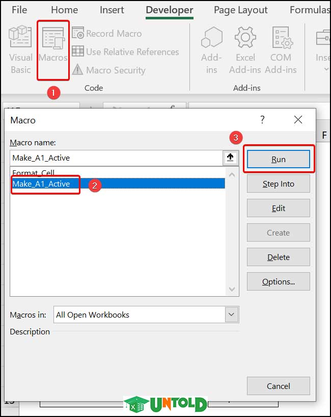
- Thirdly, close the VBA window >> click the Macros button.
This opens the Macros dialog box.
- Following this, select the Format_Cell macro >> hit the Run button.

Subsequently, the output should look like the picture shown below.

How to Make A1 the Active Cell in Excel
Sometimes you may want to make the A1 cell active, now this can be tedious if you have multiple worksheets. Don’t worry just yet! VBA has covered. Now, allow me to demonstrate the process in the steps below.
📌 Steps:
- To begin with, run Steps 1-2 from the previous method i.e., open the Visual Basic editor, insert a new Module and enter the code.
⚡ Code Breakdown:
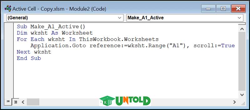
Now, I will explain the code used to make the A1 cell active.
- To start, the sub-routine is given a name, here it is Make_A1_Active().
- Next, define the variable wrksht.
- Then, use the For-Next statement to loop through all the worksheets and jump to the A1 cell using the Range property.

- Thirdly, close the VBA window >> click the Macros button.
This opens the Macros dialog box.
- Following this, select the Format_Cell macro >> hit the Run button.
Finally, your result should look like the image shown below.

Highlighting Active Cell with Excel VBA Code
Now, wouldn’t it be great if you could highlight the active cell and display its address in a cell? In order to do this, you can follow these simple steps.
📌 Steps:
- First of all, navigate to the Developer tab >> click the Visual Basic button.

This opens the Visual Basic Editor in a new window.
- Secondly, double-click on Sheet6 (Highlight Active Cell) shown in the image below.

- Next, select the Worksheet option and copy the code from here and paste it into the window.
In the code shown below, the ActiveCell property stores the Address of the active cell in the G4 cell.

- Then, exit the Visual Basic Editor and you’ll see that the G4 cell shows the address of the active cell.

- Thirdly, select the A1 cell (step 1) >> then click the Select All button (step 2).

- Now, click the Conditional Formatting option >> select New Rule.

In an instant, the New Formatting Rule wizard pops up.
- Next, choose the Use a formula to determine which cells to format option.
- Then, in the Rule Description enter the following formula.
=ADDRESS(ROW(A1),COLUMN(A1))=$G$4
- Now, click on the Format box to specify the cell color.

This opens the Format Cells wizard.
- In turn, click the Fill tab >> choose a color of your liking, for example, we’ve chosen Bright Yellow color >> hit the OK button.

Finally, the active cell will be highlighted and its address will be shown in the G4 cell.

Conclusion
This article provides the answer to what is an active cell in Excel in a quick and easy way. Make sure to download the practice files. Hope you found it helpful. Please inform us in the comment section about your experience. Keep learning and keep growing!
No comments:
Post a Comment