This article will focus on an in-depth guide about the relative cell reference in Excel. There are two types of references in excel-relative references and absolute references. Relative and absolute references behave differently when they are copied and filled with other cells. If you use relative references in a formula, the formula will change if you copy the formula to another cell. On the other hand, absolute references will remain constant, no matter in which they are copied.
What Is Relative Cell Reference in Excel?
Before understanding relative cell references, we have to understand cell references in a formula. Say we have a formula like this ‘=B3*C3+D3’. In this formula, there are three references- B3, C3, and D3. Every reference in a formula links with a cell in an excel worksheet. In other words, every cell has a unique reference. B3 can link to only one cell in the worksheet.
By default, all cell references are relative references. When you copy a formula with relative references in other cells, the references will change based on the relative positions of rows and columns. Say for example you have a formula like this: B4*C4+D4 in cell E4. Then E4=B4*C4+D4. If you copy this formula in cell E5 dragging AutoFill, then B4 will be B5, C4 will be C5 and D4 will be D5. One row down. What will be the references if you copy this formula (E4=B4*C4+D4) to cell F4? The formula will be now F4=C4*D4+E4.
Relative references are convenient when you need to repeat the same calculation across multiple columns or rows. Basically, it gets auto-updated every time we use the drag function, auto-fill feature, or copy and paste a cell.
How to Use Relative Cell Reference in Excel
In our following example, we want to calculate Menu Cost(see the heading in the example) by multiplying every menu’s price and quantity. We shall not create the formula for every cell, we shall create the formula for cell E5 and copy this formula to the other rows. Here we are using relative references.
Steps:
- First, select the cell that will contain your formula. In our example, the cell is E5 where we shall use the formula.
- Then enter your formula to calculate the desired value in the selected cell. Here, we are using the following formula.
=C5*D5
- After that, press Enter on your keyboard.
- Now select the cell again and click and drag the fill handle icon to the end of the column to replicate the formula for the rest of the cells.
As you can see from the figure all the values are calculated according to their values on the left. If you select cell E6 and look at the formula in the formula box, it will say the value is the multiplication of cells C6 and D6.
This is the power of relative cell reference. You can simply keep using cell reference and Excel will automatically replicate the formula for other cells.
Relative Cell Reference in Excel: 5 Suitable Examples
Now that we have seen the basic usage of the relative cell reference, we are going to see different examples of it and its usage. Below attached are five different examples.
1. Calculating Price with VAT from Cost
Let’s look at the following dataset.
In this dataset, we are going to calculate what will be the price after we add the VAT to the cost. For the demonstration, we are assuming there is a 5% VAT on all the products. We are going to use the relative reference here so that the cell calculations for all the cells are performed automatically.
Steps:
- First of all, select cell D5.
- Then write down the following formula in it.
=C5*1.05
- After that, press Enter on your keyboard.
- Next, select the cell again and click and drag the fill handle icon to the end of the column.
This is how you can calculate the price after VAT from cost easily using the relative cell reference in Excel.
2. Calculating Total Marks
Now let’s look at another dataset.
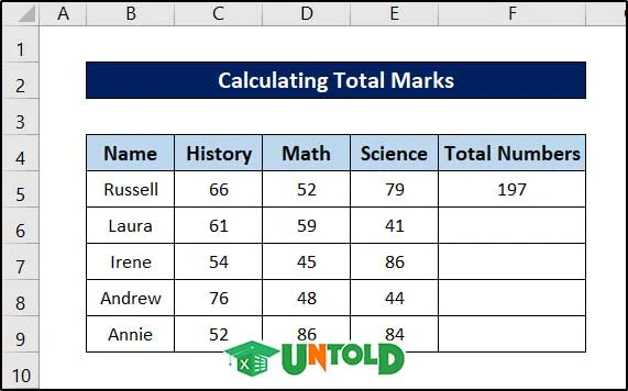
The dataset contains a number of different subjects of different persons. We are going to calculate the total number of the first person. And for using the relative reference for it, we will see that we can replicate the formula for the rest of them without repeating it.
Steps:
- First, select cell F5.
- Second, put down the following formula in the cell.
=C5+D5+E5
- Third, press Enter on your keyboard.
- Finally, select the cell again and click and drag the fill handle icon to the end of the column to replicate the formula.
This is another example of using relative cell reference to automatically replicate formulas in Excel.
3. Calculating Average from Numbers
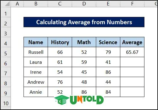
In the next example, we are going to calculate the average of numbers from the same dataset using the relative reference. As we are using the relative reference, all the cells will contain the relevant cell references. Follow these steps to see more.
Steps:
- First, select cell F5.
- Then write down the following formula in it.
=(C5+D5+E5)/3
- Now press Enter on your keyboard.
- Next, select the cell again. Then click and drag the fill handle icon to the end to replicate the formula for the rest of the cells.
We can see that all the cells now have the relevant formula because of using the relative cell reference on the Excel spreadsheet.
4. Determining Status of Age
Next up, we are going to use a formula containing a function, that will contain a relative reference. And because of using so, we will see that we can replicate formulas with their respective references.
We are going to use the following dataset to determine whether people in the dataset are adults or not.
We are going to use the IF function for this. Follow these steps to carry out the operation.
Steps:
- First, select cell D5.
- Then write down the following formula.
=IF(C5<18,"No","Yes")
- After that, press Enter.
- Now select the cell again and click and drag the fill handle icon to the end of the column to replicate the formula.
This way we can automate formulas with functions too using the relative cell reference in Excel.
5. Calculating Increased Salary from Basic Salary and Increment
Finally, let’s look at another example of the usage of relative reference in Excel. Let’s take the following dataset.
Follow these steps to see how to calculate the increased salary with their relevant cell references automatically.
Steps:
- First, select cell E5.
- Then write down the following formula.
=C5*(1+D5)
- Next, press Enter.
- Finally, select the cell again and click and drag the fill handle icon to the end of the column to replicate the formula for the rest of the cells.
Thus the increased salary can be calculated with the help of the relative cell reference in Excel.
Keyboard Shortcut for Relative Cell Reference
There is a keyboard key to toggle between relative and absolute cell references. Although not practical in most cases, you can press the key F4 to toggle from a relative reference to absolute reference to relative column and absolute row to absolute column and relative row.
For example, let’s select a cell and write down =B4 in it. By default, this is the relative reference. If you press F4 now, it will be =$B$4 in the cell. This is an absolute reference. After pressing F4 again, it will be transformed into =B$4. If we replicate this formula now, the column reference will change and the row reference will be fixed to 4. Now, if you press F4 again after that, the formula will be =$B4. This time, the column reference will be fixed and the row number will change with each replication.
If you press F4 again from this point onwards, this pattern will repeat.
Relative Cell Reference in Excel OFFSET Function
We can use the OFFSET function with both relative and absolute references. But this is one function that benefits more with the relative reference. The function can take in several arguments. Of them, a cell reference, row, and column are the primary ones. Then the function returns the value below the row number and the number of columns on the right from the reference. It can also take secondary arguments like how many rows and columns it should return.
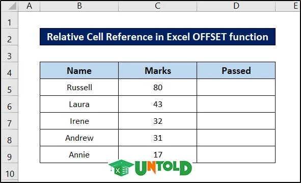
Let’s take the following dataset.
Now follow these steps to use the OFFSET function in it to determine whether someone passed or not.
Steps:
- First, select cell D5.
- Then write down the following formula.
=IF(OFFSET(B5,0,1)>32,"Yes","No")
🔎 Breakdown of the Formula
IF(OFFSET(B5,0,1)>32,”Yes”,”No”)
👉 OFFSET(B5,0,1) portion of the formula returns the value of the cell that is zero rows down and one row right of cell B5. Which, in turn, is the value of cell C5.
👉 The OFFSET(B5,0,1)>32 is the logical test of the IF function. If the number returned from the OFFSET portion is larger than 32, it returns TRUE. Otherwise, it returns FALSE.
👉 Finally, the IF function returns the string “Yes” in case the logical test returns true, otherwise it returns “No”.
- After that, press Enter.
- Now select the cell again and click and drag the fill handle icon to the end of the list to replicate the formula for the rest of the cells.
As we can see the OFFSET function uses a relative reference here. For this, whenever we move on to the next cell the cell reference of the function changes accordingly. This helps keep up with the sequence we need in the dataset.
Conclusion
That concludes our discussion on the relative cell reference in Excel. Hopefully, you have grasped the usage of the relative cell reference fully. I hope you found this guide helpful and informative. If you have any questions or suggestions, let us know in the comments below.


No comments:
Post a Comment