Working on different types of text is very common in Excel. But sometimes we need to split them for the need of better understanding. In this article, we will learn about splitting text in Excel with 8 applications.
Splitting Text in Excel: 8 Useful Applications
For illustration, here is a dataset with information on the names and addresses of 5 persons living in different countries.
Now let’s follow the examples below to split text in this dataset.
1. Use Column Wizard to Split Text in Excel
This first method will guide you on splitting text with the help of Text to Column Wizard identifying the Delimiter. Let’s check the process below:
In the beginning, go to the Data tab and select Text to Columns under the Data Tools group.
- Select the Delimited option in the first step of the Text to Column Wizard window and press Next.
- Next, select the Delimiters as Comma and press Next.
- In the last step, provide the Destination as cell C5 and press on Finish.
- That’s it, we have our split text as the following image.
2. Split Text with Flash Fill in Excel
Flash Fill is a good supplement to Column Wizard for splitting text in Excel.
- First, type the first part of your text based on cell B5 in cell C5.
- Go to the Data tab and select Flash Fill under the Data Tools group.
- You will see that range C6:C9 is automatically filled with the first part of text from each of its sources.
- Follow the similar procedure and you will get the final output.
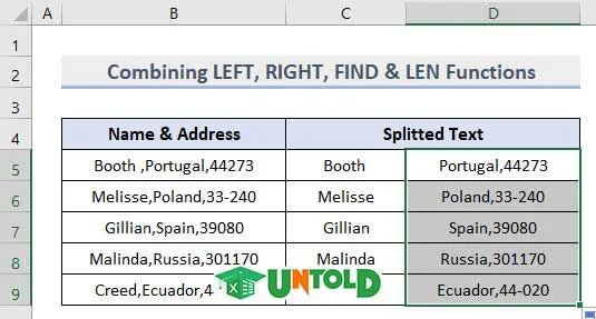
3. Combine LEFT, RIGHT, FIND & LEN Functions for Splitting Text
Another helpful method to split text is combining the LEFT, RIGHT, FIND & LEN functions in Excel.
- First, insert this formula in cell C5.
- Then, press Enter.
- Use the AutoFill feature to expand the formula and you will get the result below.
Here, we applied the LEFT function to fetch data from the leftmost side of the cell. Following, we used the FIND function to search for that text position in cell B5.
- Now, insert this formula in cell D5.
- Next, hit Enter.
- Similarly, use the AutoFill tool to get the split text in the range D5:D9.
Here, we applied the RIGHT function to extract text from the right part of cell B5. Then, we used the LEN function to define the length of the text string. Lastly, applied the FIND function to search for the specific text string.
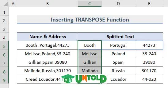
4. Insert TRANSPOSE Function for Splitting
The TRANSPOSE function is also very helpful for splitting text. Following is the process:
- Firstly, insert this formula in cell C5.
- Press Enter and you will see that the text is automatically divided into cells C5, D5, and E5.
Here, we used the TRANSPOSE function to create an array for splitting the text. Then, we insert the FILTERXML function for extracting individual items from cell B5. Lately, we used the SUBSTITUTE function to replace text based on the dataset.
- Finally, use the Fill Handle tool for the following cells.
You can also use this formula instead.
=FILTERXML(""&SUBSTITUTE(B3,","")&"", "//s")5. Apply Excel VBA to Split Text
Excel VBA is an excellent solution to split text in Excel. Let’s check the simple steps below:
- Go to the Developer tab and select Visual Basic from the Code group.
- Then, select Module from the Insert section.
- After that, insert this code on the blank page.
- Click on Run Sub/UserForm or press F5 on your keyboard.
- Next, click on Run in the Macros window.
- Finally, you have successfully done the splitting of text in Excel.
6. Use Power Query for Splitting Text in Excel
Another useful method to split text is to use the Power Query in Excel. This tool helps to import and connect to an external workbook and reshape it according to preference.
- First, go to the Data tab and select Get Data.
- Select From File and then From Excel Workbook under the context menu.
- Open the "Splitting_Text" file.
- Select the Power Query worksheet in the list of the Navigator.
- Then, press Transform Data.
- After that, go to the Transform bar and click on Split Column.
- Thereafter, select By Delimiter from the drop-down.
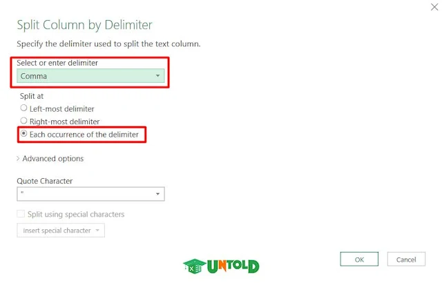
- You will be directed to the Split Column by Delimiter dialogue box.
- Here, select the delimiter as the Comma.
- Along with it, select the option Each occurrence of the delimiter to Split at section.
- Press OK.
- Lastly, press on Close & Load.
- You will see a new worksheet where the texts are split.
You can modify this table according to your preference afterward.
7. Text Splitting with TEXTBEFORE & TEXTAFTER Functions
In this method, we will describe the process using the TEXTBEFORE and TEXTAFTER functions in a new dataset. Here, it shows the information of 5 persons’ full names in range B5:B9. Let’s check the steps below.
- Insert this formula in cell C5 and hit Enter.
Here, the TEXBEFORE function is used to return the text in cell B5 before any delimiter.
- Apply this formula in cell D5 and press Enter.
Here, the IFERROR function is applied to return a value in the formula that specifies any error. Following we used the TEXTBEFORE and TEXTAFTER functions to return the text in cell B5 before and after any delimiter respectively.
- Lastly, apply this formula in cell E5.
Here, the TEXAFTER function is used to return the text in cell B5 after any delimiter.
- Now, you will see the output of cell B5.
- Lastly, use the Fill Handle tool and get the final output.
8. Split Text from a Line Break in Excel
In this section, we will discuss a new aspect of splitting text. Here, we will see the process of splitting text from a line break.
- First, insert this formula in cell C5.
We use the LEFT function to extract the left-side value. Then the SEARCH function returns the position as a number in the text string. Lastly, we used the CHAR function to return a character specified by a number in cell B5.
- Then, apply this formula in cell D5.
Here, the MID function is used to fetch the value from the middle line in cell B5. Then applied the SEARCH function to return the position in the text string. Lastly, we used the CHAR function to return a character specified by a number.
- Insert the following formula on cell E5.
First, we applied the RIGHT function to extract the right side value. Then applied the SEARCH function to return the position as a number in the text string and the LEN function to determine the length of that string. Lastly, we used the CHAR function to return a character specified by a number in cell B5.
- Here is the output against cell B5.
- Follow the same procedure and you will see the final set of split text.
How to Split Numbers from Text in Excel
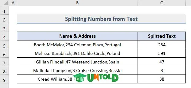
The following image shows a worksheet with some numbers and text in a single column. Our goal is to extract the number part from each cell and put these numbers into a separate column using the Flash Fill tool.
- In the beginning, insert the number of cell B5 inside cell C5.
- Then, click on the immediate next cell.
- After that, go to the Data tab and select Flash Fill.
- That’s it, you will get all the numbers at once.
Download Practice Workbook
Get this sample file and try it yourself.
Conclusion
So far, we have discussed the process of splitting text in Excel with 8 practical applications. Try them and let us know your feedback. Keep an eye on our website for more Excel blogs.


No comments:
Post a Comment